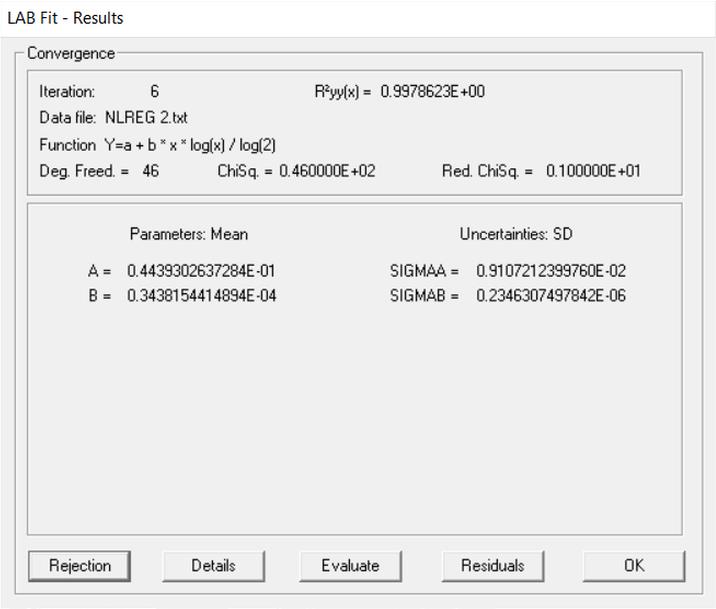
Residuals button: displays the scatter plot of residuals, including the result of the Durbin-Watson test. Presented below are typical values for the Durbin-Watson test and the corresponding residual scatter plots for three proposed fits (curve-fitting tolerance: tol = 1.0E-06). The mentioned datasets are available in the LAB Fit software.
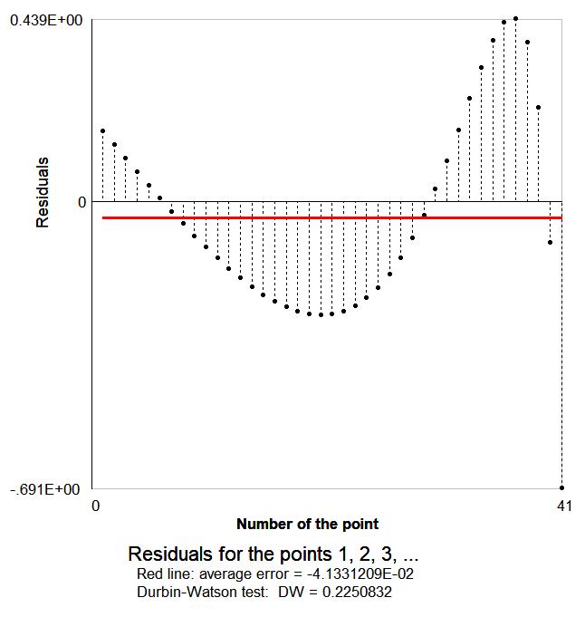
1. Positive autocorrelation of residuals (DW test close to or equal to 0.0)
Residuals of the same sign cluster together. If a residual is positive, the next one is very likely to be positive as well, creating a "wavy" or "cyclical" pattern. See the example below, resulting from fitting function number 17 to the dataset "DW test almost 0 (function n. 17).txt":
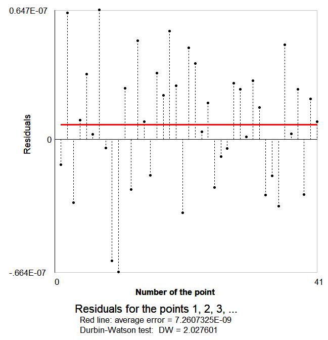
2. No autocorrelation of residuals (DW test close to or equal to 2.0)
The residuals are completely independent. Knowing the sign of a residual makes it impossible to predict the sign of the next one. See the example below, resulting from fitting function number 11 to the dataset "DW test close to 2 (function n. 11).txt":
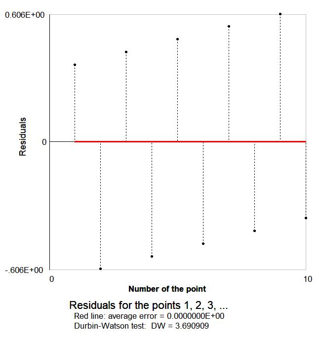
3. Negative autocorrelation of residuals (DW test close to or equal to 4.0)
Residuals constantly alternate signs. A positive residual is immediately followed by a negative one, and vice versa. See the example below, resulting from fitting function number 6 to the dataset "DW test almost 4 (function n. 6).txt":
Note: In simplified terms, DW values between 1.5 and 2.5 are generally considered "acceptable" or "normal" in curve fitting, presenting no cause for concern. For values significantly outside this range, the curve fit should be critically evaluated and the causes identified. After that, the user can decide whether or not to be tolerant.
Example: Based on the DW test, could function number 102 (obtained with LAB Fit Finder, DW = 1.8829) better represent the dataset "DW test almost 0 (function n. 17).txt" than function number 17 (DW = 0.2251)?
Answer: The new scatter plot of residuals is shown below (function number 102):
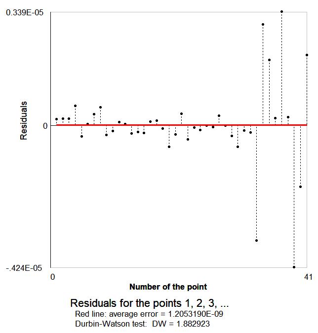
So, from the perspective of the DW value, the answer is yes: function number 102 represents the mentioned dataset* better than function number 17.
*The dataset used in this example was generated through a 4th-order Runge-Kutta method (RK4, with single precision, 41 points) numerical integration of the differential equation dy/dx = y x2 (with x0=1; xf=2 and y(x0)=2). Consequently, the residuals presented by the analytical solution found by LAB Fit (function number 102) correspond to the deterministic truncation errors of the RK4 method rather than random sampling noise. The magnitude of these errors increases toward the end of the interval due to the exponential growth of the solution. The DW value equal 1.8829 confirms that the LAB Fit "Finder" tool successfully retrieved the true underlying analytical model, leaving only the numerical artifacts of the simulation as residuals. Please see below function no. 102 fitted to the points of the numerical solution:
